What is linear algebra?
A branch of mathematics that studies the properties of vector spaces and linear maps. It deals mainly with matrices, vectors, and systems of linear equations, and is widely applied in various fields of science, engineering, and economics.
Linear
The term “linear” refers to the property of having a certain linearity. Specifically, a function or mapping is called linear if it satisfies the following conditions
- Closed to addition: f(x+y)=f(x)+f(y)
- Closed to scalar doubling: f(cx)=cf(x)
Functions and maps that satisfy these properties are called linear, and models and equations using them are called linear equations.
A linear function is a linear function. Higher dimensional versions of linear functions are functions by matrices, linear functions.
Quadratic and trigonometric functions are nonlinear functions
Algebra
Algebra is the branch of mathematics that deals with generalized operations on numbers and quantities. Basic algebra operations include addition, subtraction, multiplication, and division. Algebra uses numbers as well as letters and symbols to represent mathematical expressions, and uses a variety of laws to perform calculations and operations. The purpose of algebra is to manipulate mathematical expressions to find solutions and to understand the structure of expressions.
In linear algebra, these algebraic concepts are applied to vectors and matrices to investigate operations and relationships within vector spaces. Concepts such as computation with matrices and the basis, dimension, and orthogonality of vector spaces play an important role.
Vector
- Some combination of numbers, representing quantities with magnitude and direction
Matrix
- Numbers are arranged in rows and columns. Vectors are also part of a matrix.
- The product of matrices transforms a vector X into another vector y=Ax. Matrices allow scaling, flipping, rotating, and shearing to be represented.
Applications of Linear Algebra
Computer Science and Machine Learning
- Matrices and vectors are widely used in the representation and manipulation of data and in the design of algorithms.
- Machine learning models (e.g., neural networks) process input data using a weight matrix.
physics
- Represent physical quantities such as force, motion, and electric and magnetic fields using vectors and matrices.
- In quantum mechanics, state vectors and matrix operations play an important role.
economics
- Use matrices and vectors in solving economic models and optimization problems.
- For example, input-output analysis uses a matrix representation of transactions between industries.
Graphics and Image Processing
- Matrix transformations are used in 3D graphics rendering and image filtering
- Represent geometric transformations such as affine and projective transformations in terms of matrices.
systems engineering
- In control theory, state vectors and transfer matrices are used to describe system behavior.
- In robotics, the position and posture of a robot are represented by vectors and matrices.
(the study of) statistics
- Multivariate analysis treats data as a matrix and applies methods such as principal component analysis and factor analysis.
- In regression analysis, the parameters of the model are also estimated using matrix operations.
Simplify a differential equation, which is a continuous problem, by discretizing it by expanding it to the limit and treating it as a straight line with numbers, so that it can be solved by linear algebra
Discretization of differential equations
- Differential equations express continuous changes of a function, which can be discretized and solved numerically by using the finite difference method (continuous changes of a function are approximated by finite differences) or the finite element method (the domain is divided into small elements, and the function is approximated within each element). Discretized differential equations often take the form of simultaneous linear equations, which can then be expressed in matrix form and solved using linear algebra.
Properties of matrix operations
- The combining, exchange, and distributive laws are the same as for ordinary numbers.
- Product is not commutative (non-commutative): AB ≠ BA →, Unlike ordinary numbers, we need to distinguish between “multiply from the left” and “multiply from the right”.
line base transformation
Literally, the basic operations performed on the rows of a matrix. Using these operations, matrices can be transformed into a simple form, which is useful for solving linear systems of linear equations and for finding the factorial of a matrix. There are three types of row-basis transformations
- Row swap: swap two rows; Ri↔Rj
- Row constant multiply: multiply a row by a non-zero constant, Ri→kRi
- Add/subtract rows: add a constant multiple of another row to one row; Ri → Ri + kRj
Although column basis deformations can be defined in the same way as row basis deformations, row basis deformations are often used in terms of inconvenience in solving simultaneous equations and computing matrix rank and inverse matrices.
Sweep method (Gaussian elimination method)
A method of converting a matrix to a staircase matrix (upper triangular matrix) using row basis transformations. This method is used to solve simultaneous linear equations and to find the factorial and inverse of a matrix.
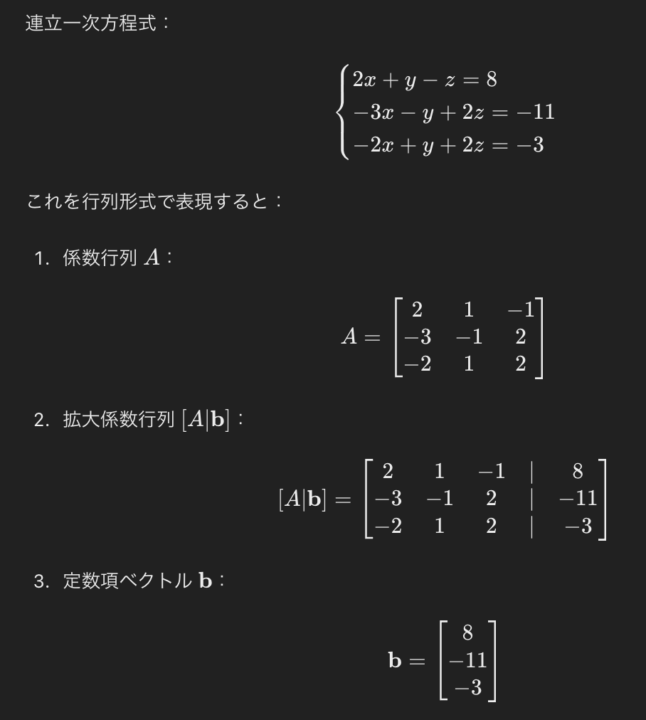
Coefficient matrix: A matrix of linear simultaneous equations with only the coefficients taken out and expressed as a matrix.
Constant term vector: A vector created by collecting the constant terms on the right-hand side of a simultaneous linear equation. Equivalent to the right-hand side of each equation.
The expanded coefficient matrix is a matrix that is expanded by adding a constant term vector to the coefficient matrix. This allows the entire simultaneous linear equations to be represented by a single matrix

Whether the solution of a simultaneous equation is uniquely determined, an indefinite solution is obtained, or there is no solution (impossibility) depends on the rank of the expansion coefficient matrix and the rank of the coefficient matrix.
Relationship between rank and unique, indefinite, and indefinite/non-unique
Matrix rank denotes the intrinsic dimension of the matrix and the number of independent equations. The number of nonzero rows when the matrix is transformed into a staircase matrix by row basis transformation.
For n-dimensional simultaneous equations
narrow view
- rank(A) = rank[A|b] and n = rank(A)
- When the ranks of the coefficient matrix A and the expanded coefficient matrix [A∣b] of a simultaneous linear equation coincide and their ranks coincide with n
Indefinite (solution not determined)
- rank(A) = rank[A|b] and n > rank(A)
- When the ranks of the coefficient matrix A and the expanded coefficient matrix [A∣b] of the simultaneous linear equations coincide and their ranks are smaller than n
Impossibility (no solution exists)
- rank(A) ≠ rank[A|b].
- When the ranks of the coefficient matrix A and the expanded coefficient matrix [A∣b] of a simultaneous linear equation do not match
determinant
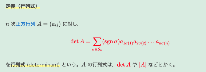
The determinant is a number that is defined as follows for a square matrix (a matrix with the same number of rows and columns).
The determinant of matrix A is denoted as det(A) or |A|.

Substitution and Compatibility
Substitution: An operation to reorder the elements of a set in a specific order.
Compatibility: Among substitutions, those that only exchange two elements; are written as (i,j) for compatibility that exchanges i and j.
odd and even replacements
Whether a substitution is an odd or even substitution depends on the number of compatibilities needed to perform the substitution.
- Even Substitution: Substitution that can be represented by an even number of interchanges.
- Odd substitutions: substitutions that can be represented by an odd number of interchanges.
For example, the substitution (1,3,2) for the set {1,2,3} is odd substitution because it can be represented by one substitution (2,3). On the other hand, substitution (3,2,1) is an even substitution since it can be represented by two interchangeable (1,3) and (1,2).
The Sign of a Permutation is a number that indicates whether the substitution is an odd or even substitution, and is defined as follows
- For even substitution, sign sgn(σ)=+1
- For odd substitutions, sign sgn(σ) = -1
Properties of the determinant derived from the above definition
- Transpose invariance: the determinant of a matrix is equal to the determinant of its transpose matrix. det(A) = det(At)
- Alternativity: When the rows or columns of a matrix are swapped, the value of the determinant is multiplied by -1.
- Multilinearity: adding a constant multiple of one row (column) to another row (column) does not change the value of the determinant
- det(A)≠0 ⇔ there exists an inverse of A (A is regular)
- In 2- or 3-dimensional space, the determinant represents the volume (or area) of a parallelepiped or parallelogram
- Scaling Linear Transformations: A matrix represents a linear transformation. The value of the determinant indicates how much the transformation scales up or down the volume (or area).
Inverse Matrix: For a regular matrix, an inverse matrix is a matrix that when multiplied by its matrix becomes a unit matrix.
Cofactor expansion: A method of computing the determinant of a matrix that uses cofactors corresponding to specific elements.
Mi, j is the (i, j )-submillimetric determinant of A, i.e., the determinant of the (n – 1)-order small square matrix obtained from A excluding the i-th row and j-th column

For example, the cosine factor expansion based on the first row of matrix A is expressed as This can be computed based on other rows or columns of the matrix as well.
Eigenvalues and eigenvectors
(Definition) For an nth-order square matrix A, a scalar 𝜆 satisfying Ax=λx (x≠0)𝐴𝑥=𝜆𝑥 (𝑥≠0) is called an eigenvalue of A, x∈Rn being an eigenvector corresponding to 𝜆.
Normally, applying an nth-order square matrix A to a vector changes the vector’s orientation, but for certain vectors, the orientation may not change when A is applied, and such special vectors are called eigenvectors. In such cases, the number of times the length of the eigenvector is called the eigenvalue.
How to find eigenvalues and eigenvectors
(1) Derivation of eigen equations Eigenvalues are obtained as solutions of the following eigenequations: det(A-λE)=0
E is the unit matrix. Solve the above equations to obtain the eigenvalues λ.
(2) Solution of eigenvector Once the eigenvalue λ is obtained, the corresponding eigenvector x is found by solving the following linear equation (A-λE)x=0
matrix diagonalization
- For a given square matrix A, there exists a suitable regular matrix P, making P-1AP a diagonal matrix D (a matrix whose non-diagonal components are all zeros).
- The matrix can be diagonalized only when the eigenvectors of A have n linearly independent eigenvectors, and the diagonal components of the resulting diagonal matrix are the eigenvalues of A.
If one wants to find the n-square of matrix A, it is difficult to calculate it as it is, so it can be easily obtained by first diagonalizing the matrix (if it can be diagonalized) and then using the n-square of the diagonal matrix D.
Jordan standard form (quasi-diagonalized)
If A has overlapping eigenvalues (heavy solution), it may not be diagonalizable, in which case the Jordan standard form is used.
It was born out of the motivation to make it as easy as possible to find the nth power of A, even when it cannot be diagonalized.
A Jordan block (Jordan cell) is a matrix with the same value λ in the diagonal components and 1 in one upper part. All other components are 0. Write J(λ,k) using the diagonal component λ and the matrix size k. For any matrix A, the Jordan standard form is uniquely determined (except for the arbitrariness of the order of the blocks).


